Tabsets
The Tabsets application demonstrates using tabs to organize output. To run the example type:
library(shiny)
runExample("06_tabsets")
Tab Panels
Tabsets are created by combining nav_panels()s in a navigation container. The bslib package provides many styles of navigation containers, including:
navset_underline()andnavset_card_underline()navset_tab()andnavset_card_tab()navset_pill_list()navset_pill()andnavset_card_pill()navset_hidden()navset_bar()
Each allows the user to navigate the panels in a different way. Functions that contain card in their name place the navigation container within its own card.
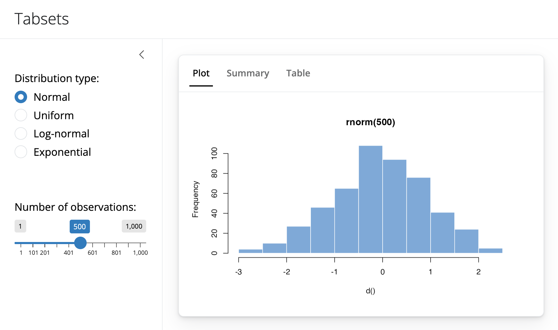
In this example, we added a summary and table view of the data to the Hello Shiny app, each rendered in their own panel. We combined the panels with a navigation element that underlines the name of the active tab. Here is the source code for the UI object:
library(shiny)
library(bslib)

# Define UI for random distribution app ----
# Sidebar layout with input and output definitions ----
ui <- page_sidebar(

  # App title ----
  title ="Tabsets",

  # Sidebar panel for inputs ----
  sidebar = sidebar(

    # Input: Select the random distribution type ----
    radioButtons("dist", "Distribution type:",
                 c("Normal" = "norm",
                   "Uniform" = "unif",
                   "Log-normal" = "lnorm",
                   "Exponential" = "exp")),
    # br() element to introduce extra vertical spacing ----
    br(),
    # Input: Slider for the number of observations to generate ----
    sliderInput("n",
                "Number of observations:",
                value = 500,
                min = 1,
                max = 1000)
  ),

  # Main panel for displaying outputs ----
  # Output: A tabset that combines three panels ----
  navset_card_underline(
    title = "Visualizations",
    # Panel with plot ----
    nav_panel("Plot", plotOutput("plot")),

    # Panel with summary ----
    nav_panel("Summary", verbatimTextOutput("summary")),

    # Panel with table ----
    nav_panel("Table", tableOutput("table"))
  )
)
Building a tabset is very similar to building a multi-page app. Instead of passing nav_panel()s to page_navbar(), we instead pass them to a navigation container. Also, just as with a multi-page app, we can use bslib’s nav_spacer(), to control the alignment of UI elements in the tabset’s navbar, and nav_item(), to add items to the navbar, such as an html link.
Tabs and Reactive Data
Introducing tabs into our user interface underlines the importance of creating reactive expressions for shared data. In this example, each tab provides its own view of the dataset. If the dataset is expensive to compute then our user interface might be quite slow to render. The server function below demonstrates how to calculate the data once in a reactive expression and have the result be shared by all of the output tabs:
# Define server logic for random distribution app ----
server <- function(input, output) {

  # Reactive expression to generate the requested distribution ----
  # This is called whenever the inputs change. The output functions
  # defined below then use the value computed from this expression
  d <- reactive({
    dist <- switch(input$dist,
                   norm = rnorm,
                   unif = runif,
                   lnorm = rlnorm,
                   exp = rexp,
                   rnorm)

    dist(input$n)
  })

  # Generate a plot of the data ----
  # Also uses the inputs to build the plot label. Note that the
  # dependencies on the inputs and the data reactive expression are
  # both tracked, and all expressions are called in the sequence
  # implied by the dependency graph.
  output$plot <- renderPlot({
    dist <- input$dist
    n <- input$n

    hist(d(),
         main = paste("r", dist, "(", n, ")", sep = ""),
         col = "#007bc2", border = "white")
  })

  # Generate a summary of the data ----
  output$summary <- renderPrint({
    summary(d())
  })

  # Generate an HTML table view of the data ----
  output$table <- renderTable({
    d()
  })

}You can access the name of the currently active nav_panel() as a reactive variable. To do this, pass an optional id argument to the navigation container, e.g. navset_card_underline(id = "tab", ...). The name will be available in reactive contexts as input$<id>, e.g. input$tab.